Whitepaper
The Most Basic Lessons of Investing
By Stan Miranda
30 September 2013
This note describes the most important learning about investing including some very basic principles and some useful tools. Many of these are rooted in fundamental academic research, and generally accepted. A few are only supported by what we believe to be compelling common sense. We would expect that the most sophisticated and successful institutional investors embrace these principles wholeheartedly and use these tools. We would expect all of our clients to find this learning valuable, regardless of how sophisticated. We have chosen 8 core lessons for this note from among the hundreds which we follow and use every day. These 8 lessons from the platform of beliefs that underpin portfolio strategies for every one of our clients and include the following:
- There is no return without risk
- Economic cycles and risk
- Permanent declines vs. temporary “paper” losses
- A common measure of investment risk: Standard Deviation of returns
- Benefits of diversification
- Long term investors’ advantages over short term investors
- Market returns (beta) vs. manager excess returns (value added or alpha)
- The futility of market timing
1. There Is No Return Without Risk
The first and most important principle of investing is that returns are only earned by taking risk. Risk is defined as the chance that you lose some or all of your capital invested. This loss can be a decrease in the valuation of assets held (an “unrealised” loss) or it can be a permanent loss which has been realized by having sold the asset below its purchase cost. An ideal investment strategy would be to get a return without taking any risk of decline, but this simply does not exist in the real world. There are lucky investors who will not have seen the value of their assets decline for a long period after investment, but the risk of their decline is always present. Investment returns only come from exposing assets to the possibility of decline.
The opposite is not true. By virtue of simply taking risk of decline, one is not guaranteed a return. There are many examples of “return-free” investment risk. A company that clearly has no chance of ever earning a profit has plenty of risk, but investing in it is certain to not pay a return to the investor. An example of return-free risk used today is US government bonds. With yields below the rate of inflation, expected real returns are negative, but there is clearly the risk that the value goes down and even that the full amount may not be paid upon maturity. These are examples of “bad” investments. “Good” investments are those that pay a return commensurate with the risk of losing money.
Investors are paid to take different types of risk. The oldest form of investment return is from lending money to borrowers. If you are the lender, the interest is paid to you for what? For taking the risk that the borrower will not repay you the principle. This is known as “credit risk.”
The next most common form of investment return comes from investing capital into companies that make products or deliver services that can be sold, ideally for more than the cost of making or delivering those products or services. The investment return paid is a dividend or pay-out of the profits from the business. What is the risk that you are taking by investing in a company? The risk is that revenues are less than costs and the resulting losses erode away your capital invested in the company and it is not returned to you in full. That is known as “equity risk”. It is the same with private companies as well as publicly listed companies. With public companies the share prices are driven not just by company profitability, but also by market forces (e.g., investor sentiment, supply and demand for shares). The risk of the public company is still that there will be no profits and therefore no dividends. But in a publicly traded equity security (shares), the price reflects fear or excitement about the future company earnings and the value may decline or rise ahead of profits rising or declining.
A third type of investment risk is interest rate or duration risk. The best example of this is government bonds or bank deposits. Before the recent global financial crisis, a US, Japanese or Portuguese government bond was viewed as very safe with no risk that you would not be paid. So there was no credit risk or a reward that has to be paid to the holder of government bonds for the risk of default or the government not paying all of the principle back when the bond matured. So what is the risk that the government is paying for when it paid 4% for 10 year bonds and 1% for a 3 month maturing bond? In the case of the 10 year maturing bond, it must pay the investor more than for a 3 month bond, to reward the investor for taking the risk that interest rates might go up and the investor would miss that opportunity to invest and earn a higher rate of interest. In the case of a 3 month maturity bond, the risk that the investor will forego the opportunity to earn higher interest if rates rise is obviously much lower because he or she can move the money in just 3 months instead of 10 years, and 3 months is much less likely to experience a large increase in interest rates. So the investor is being paid for the risk that he or she loses the opportunity to earn higher interest rates in the future. This is known as interest rate risk. It is also called duration risk as the risk goes up with the longer duration or maturity period of the bond.
The fourth risk that investors are typically rewarded for is related to the loss of purchasing power of the investors’ capital while it is being tied up. In times of high inflation, if money is deposited in a bank for one year with no interest being paid and the depositor has no access to it, and inflation ran at 10% over that one year, the real value of that money when returned to the investor is 90% of what it was; ie, the investor has lost 10% from depositing it in the bank. No one would deposit money in a bank, or invest it if it was not somehow protected from expected inflation by going up in value at least as much as inflation. Various assets which pay a return that rises specifically or generally in line with inflation are paying the investor for the risk of inflation. This applies to variable rate deposit instruments, property where rents charged typically rise with local inflation and with commodities where prices move to compensate for declines in purchasing power (ie, they track inflation). The risk being rewarded here is not credit, equity or interest rate risk, but rather inflation risk.
These are the four core risks that most investors are paid for and those identified by most investment world academics. A fifth risk that we feel we must also mention is illiquidity risk. Given two identical investments, but where one is locked away in a box for 10 years and the other can be sold to cash at any moment in time, investors will require a higher return from the investment in the box. This is referred to as liquidity risk for which a “liquidity premium” must be paid – usually an amount between 1 and 10% per annum above the return one can expect to earn on the totally liquid version of that same investment.
2. Economic Cycles and Risk (partial source: Howard Marks, Oaktree)
Economies rise and fall quite moderately (think about it: a 5% drop in GDP is considered massive). Companies see their profits fluctuate considerably more, because of their operating and financial leverage. But stock market gyrations make the fluctuations in company profits look mild. Securities prices rise and fall much more than profits, introducing considerable investment risk. Why is that so? Primarily, I think, because of the dramatic ups and downs in investor psychology.
The economic cycle is constrained in its fluctuations by the existence of long-term contracts and the fact that people will always eat, pay rent, buy gasoline, and engage in many other activities. The quantities involved will rise and fall, but not without limitation. Likewise for most companies: cost reductions can mitigate the impact of sales declines on earnings, and there is often some base level below which sales are unlikely to go. In other words, there are limits on these cycles. But there are no checks on the swings of investor psychology. At times investors get crazily bullish and can imagine no limits on prosperity, growth and appreciation. They assume trees will grow to the sky. Nothing’s too good to be true. And on other occasions, correspondingly, despondent investors can’t think of any limits to how bad things can get. People conclude that the “worst case” scenario they prepared for isn’t negative enough. Highly disastrous outcomes are considered, even likely.
The important conclusions from observing the above pattern are these:
- Over time, conditions in the real world – the economy and business – cycle from better to worse and back again.
- Investor psychology responds to these ups and downs in a highly exaggerated fashion.
- When things are going well, investors swing to excessive euphoria, under the assumption that everything’s good and can only get better.
- And when things are bad, they swing toward depression and panic, viewing everything negatively and assuming it can only get worse.
- When the outlook is good and their mood is ebullient, investors take security prices to levels that greatly overstate the positives, from which a correction is inevitable.
- And when the outlook is bad and they’re depressed, investors reduce prices to levels that overstate the negatives, from which great gains are possible and the risk of further declines is limited.
The excessive nature of these swings in psychology – and thus security prices – dependably creates opportunities of over- and under-valuation. In bad times securities can often be bought at prices that understate their merits. And in good times securities can be sold at prices that overstate their potential. And yet, most people are impelled to buy euphorically when the cycle drives prices up and to sell in panic when it drives prices down.
While buying in bad times and selling in good is the logical action if you believe that investor psychology drives prices beyond fair value, holding an investment through a full cycle may be easier to execute emotionally. The worst action of all is to buy with everyone else and to sell with everyone else.
The Zero-Sum Investment World
Sadly, most investment activity does not add value to the world. The pool of profit growth and investment value growth will be what it is regardless of what any one investor does. As such, the actions of any one investor only serve to give capital to other investors through their loss-making investments or to take capital away from other investors in the case of their winning investments. In other words, investing is a zero-sum game. The smartest investors take value away from the less smart. The psychology of investors describes the less smart investors. In the world of public securities (e.g., stocks and bonds), price movements are most dramatic when investors panic most. A panic can be panic buying in fear of missing gains or panic-selling when there is a fear of losing large amounts of money quickly. Panics happen fast in both directions. On these days of market panic, prices move the most. Periods of panic, therefore are when value is transferred from the losers to the winners. In a panic down market, panic sellers are generally selling well below intrinsic value and buyers are buying cheap. In a panic upward rally, the panic buyers are generally paying above intrinsic value and buying from the less panicked sellers who see the prices being paid are above their true value. The implication is simply to never panic and to remember that when others panic, it is a time for calm heads to take value from other investors.
“Buy on the cannons, sell on the trumpets” -Nathan Rothschild, 1810
3. Permanent Declines vs. Temporary “Paper” Losses
A loss is the difference between what you paid for an investment and what it is worth today (usually evidenced by a market price). Market prices and nonmarket prices (estimates based on formulas or third party estimators) go up and down. Permanent losses are those which have been fully realized through sale, liquidation or termination (eg, bankruptcy). Such losses have been realized and are not coming back. Theoretically you can repurchase the investment and recover this loss, but we still think of that loss as permanent and realized.
Temporary or paper losses are those that have not been realised by virtue of selling or liquidating the investment or having that investment’s life terminated. These losses have a chance of being recovered. Market prices tend to go down more than intrinsic value would suggest due to human nature which has investors panicking and moving in herds. It is the very nature of financial markets to behave in this manner such that prices routinely fall below their intrinsic or true value. Obviously the opposite is true as well; that investors move in herds and “panic-up” driving asset prices above intrinsic value.
The job of the intelligent investor is to avoid permanent losses and to accept temporary paper losses. Most investments are subject to the prospect of permanent loss. Those that are not subject to complete permanent loss are thought to be government bonds (in normal circumstances) and hard assets such as land, natural resources or commodities. Virtually all other investments are subject to permanent loss. The primary contributing characteristics of investments most subject to permanent loss are the following:
- Anything leveraged with debt – the value of the underlying asset falls below the value of the debt, the debt is defaulted on and the asset is taken away from you and given to the lender. So mortgaged property, leveraged buyouts, a public company who has borrowed too much and certain leveraged hedge funds are most vulnerable to permanent loss from leverage.
- Undiversified assets. A single company has a much greater chance of creating a situation of complete permanent loss than two companies or more. Companies can become unprofitable even without debt. A single unleveraged building can become worthless in extreme cases (natural disaster, poor location has rents below maintenance cost, etc.). Diversification reduces the prospect of permanent loss.
- Extreme riskiness to income flows. This could apply to government bonds (Argentina’s default), venture capital company start-ups, etc.
The implication here is not that investors should avoid anything that can result in permanent losses, but rather that they should demand higher returns for taking that risk. The other important implication is that temporary losses that appear to be the result of prices falling below intrinsic value should be viewed as relatively unimportant to the true long term investor. We cannot avoid accounting for and reporting unrealised temporary losses, but to the extent they are in fact temporary, they are irrelevant to the true long term investor. The most practical implication of this is that, if the presence of temporary losses is accepted as normal, one can take higher levels of exposure to an asset class such as public equities than might be indicated if one is more concerned about monthly or annual declines.
4. A Common Measure of Investment Risk: Standard Deviation of Returns
The standard deviation is exactly that – a standard or normal variation in outcomes. In the investment world, this is a measure that quantifies the normal variation or dispersion from the expected investment return. The riskier the asset, the more dispersed will be the range of normal return outcomes around the expected long term average; i.e., higher risk assets have a higher standard deviation of returns. A low standard deviation reflects potential outcomes being more closely grouped around the expected return – or safer assets. In investing, standard deviations are usually referring to an annual standard deviation around average annual returns (mean returns). But the same tool can be applied to deviations of returns covering any period of time.
The field of statistics that deploys the measure of risk in the form of a standard deviation assumes that outcomes fall in a predictable pattern that is described as a “normal” or bell-curve shaped distribution as shown below. For example, a normal distribution of future possible returns with an expected return of +8% and a standard deviation of 14%, arrives at a range of outcomes with probabilities attached to them as shown below by the area under the curve between one and two standard deviations.
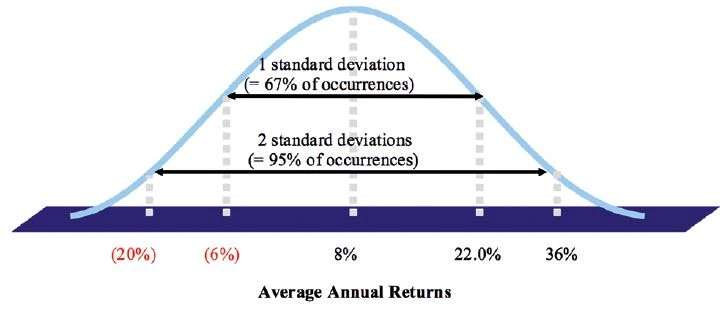
A normal bell-curve is defined as one where one standard deviation above and below the mean captures 2 out of every 3 year’s returns (67% of occurrences). In this example, it suggests that in 2 out of every 3 years, returns will be between -6% to +22.0%, a one-standard deviation range around the mean. The same normal distribution implies that there are smaller probabilities of more extreme outcomes. The range of outcomes defined by two standard deviations above and below the mean captures the outcomes in 19 out of 20 years (or 95% of occurrences). In other words, in 1 out of 20 years, the outcome would be greater or less than the range defined by two standard deviations. Just looking at the downside outcome (ie, two standard deviations below the mean, we expect this to happen in 1 out of 40 years (2.5% of the time). In the example above, this says that an annual return of -20% should only happen in one out of 40 years.
Financial assets return outcomes will not necessarily follow a normal or bell-curve shaped distribution. However, in the absence of evidence to the contrary, this distribution is often presumed to be the most likely.
Standard deviation of returns is a good long-term measure of portfolio risk and helps quantify risk versus return for different asset classes and portfolios constructed around such asset classes. In particular, standard deviation is a useful tool for assessing future downside risk.
However, standard deviation is not useful as an ongoing portfolio risk management tool. Asset volatility can vary significantly in short periods of time, depending on the market environment. The measure tends to increase during times of downward stress implying that portfolio risk will need to be reduced at precisely the wrong time, missing gains from subsequent market recovery. This is the opposite of long term investing.
Risk is better measured in terms of the portfolio’s value movement with, or in relation to, the market’s value. This relationship is measured by the factor that captures the proportion of portfolio value change as a percentage of the market’s value change. This factor is referred to as the “beta” to the market. Beta merely means value movement relative to the market’s value move. For example, a portfolio with a beta to equity markets of 0.6 can be expected to rise 6% when equity markets have gone up 10% in a period. The market beta of each asset or fund in a portfolio can simply be summed up across the portfolio to give an excellent measure of overall portfolio risk or “exposure”. By tracking underlying fund and asset betas each month we can always know the portfolio’s overall risk level and use this information to regularly rebalance portfolios back in line with targeted risk levels. This is a huge advantage as it removes a classic source of performance “leakage” from inadvertent market timing (i.e., selling low, buying high).
5. Benefits of Diversification
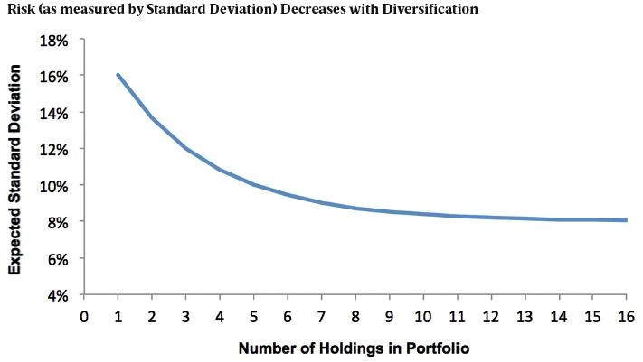
The range of possible returns from one investment are much broader than the range of possible returns from a larger number of investments, especially if the large number of investments’ returns are determined by different things. The essence of diversification is about holding sufficient number of different investments whose returns are influenced by different factors. You can see below that the benefits of diversification are greatest as you move away from a single stockholding to two and then risk (standard deviation) diminishes considerably after holding about 12 stocks from different industries.
The benefits of diversification can be further enhanced by not just diversifying within an asset class (such as the above example which diversifies between different stocks within the Public Equities asset class) but by also diversifying between asset classes. Risk adjusted returns can be improved within a portfolio by combining different asset classes, to the extent that those asset classes do not move in the same way (i.e. have a low correlation with each other).
Multi asset class diversification is best thought of by first considering equities and government bonds. These two assets typically move in opposite directions: public equities gain in value when economies are expanding and interest rates are rising, whereas government bonds typically gain in value in times of crisis when capital flows towards the safest investments. Hence these two assets can be expected to have a degree of negative correlation. By combining public equities and government bonds in a portfolio, an investor can protect against the downside of weak economic growth but still participate in the upside. This is the essence of multi-asset class diversification as practiced by the US endowments and most famously by David Swensen at the Yale Endowment.
Multi-asset class diversification can be extended from public equities and government bonds to a wide range of other investments such as property, commodities and credit. Each of these asset classes has a differing level of association with the four main risks identified at the start of this document. For example, property tends to correlate with the risk of inflation as periods of high inflation tend to result in rents charged rising with local inflation. By optimising a diversified portfolio of different asset classes, an investor can achieve a higher level of return for a given risk than could be achieved by holding just one single asset class (eg, equities). This improvement in risk adjusted returns (returns delivered for the amount of risk taken) is measured by the Sharpe ratio which is defined as the amount of return above that earned by cash deposits divided by the level of risk (as measured by the standard deviation of returns). Diversification improves the Sharpe ratio of a portfolio.
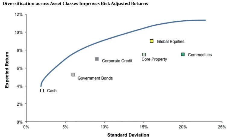
The blue line above is known as the “efficient frontier” and defines the return achieved (vertical axis) from the optimal mix of asset classes for any given level of risk (standard deviation on horizontal axis). So if the investor would like to limit the annual standard deviation to say 10%, the most optimal mix of asset classes at this risk level would be expected to generate a 9% return on average. You can see that no one asset class falls on the efficient frontier (other than cash at point where there is almost no risk being taken). This is because the asset classes are not highly correlated with one another and the combining of assets always generates more return for the same risk. This is often referred to as the “free lunch” from multi-asset class diversification; i.e., the investor gets more return for the same risk level of a single asset class. This tool is used by most portfolio managers to construct the optimal multi-asset class portfolio and was designed initially by Professor Markowitz and is referred to as his mean –variance optimization model. The obvious limitations of this model are the accuracy of the inputs which are future estimates of asset class return, standard deviation and cross asset class correlations. A heavy dose of judgment is ideally deployed on top of the use of this tool in arriving at a target asset allocation.
6. Long-Term Investors’ Advantages Over Short-Term Investors
Sadly, investing as an activity on its own generally does not add value to the world. The exception may be property development or private equity where investors are using their money to build properties or companies to enhance the growth of the economy. Being a lender may also add value as people can borrow to spend more and grow the economy (up to a limit). But the purchase and sale of public equities, bonds, commodities, and mature properties creates no value by itself. Investing is therefore often referred to as a “zero-sum game” where there are only winners and losers, but at the end of all the buying and selling, the economic pie has not grown; it has only been redistributed. So active investing is about taking value away from other investors. It is a highly competitive battlefield to do exactly that. The vast majority of the investors in the world are professionals who are paid to win at investing and they care hugely about their short term earnings, not their long term earnings. They want bonuses this year, not 5 or 10 years from now. They have mortgages and school fees to pay today. The personal investors are equally short term in their thinking. They are mostly unsophisticated investors who judge themselves on what worked this week, month or maybe year. They struggle to think longer term. So the battlefield where perhaps 90% of the investment world is competing to gain a share of the pie is very short term. For that reason alone, a wise investor would focus on the long-term. It is just less competitive. Very few people are investing for 5 or 10 year horizons, so it should just be easier to win on that battlefield. And who are the losers in the long term battle? The short term investor. The basic rule of out-performance in investing is that long-term investors take from short term investors. This is how it works in practice.
In any one calendar year, you will have noticed that the majority of the big market price moves (thinking about the stock market) that add up to the full years’ performance happen on a small number of days during the year. And in extreme performing years, the majority of the price movement happens in a small series of sequential days where there is a panic driving prices up, or a panic (fear of missing out) driving prices up. This is human nature. But who are the buyers and who are the sellers during those few important days? The sellers in a panic are the short term investors who care hugely about this year’s bonus or performance review with their boss or the entrepreneur who worked very hard to make the money he just doesn’t want to lose. The entrepreneur calls his broker (who makes a commission from buying and selling often) and asks him what he should do. He sells. Who buys? The long term investor. The patient active deep research oriented equity manager who knows the company inside out and knows the price just fell below the intrinsic value of the company. He knows, in the long term, the stock price will go higher. In that moment, the short term investor hands out-performance to the long term investor.
Another reason the long term investor wins over the short term investor is because long term outcomes are often easier to be right about than short term ones. Will Apple win the tablet war is a long term question. It is far from 100% certain, but perhaps 70% certain. Will Apple have a positive surprise on quarterly earnings? Will iPhone 5 sell as many phones this Christmas as is expected? These are difficult short term questions that short term investors love to bet on. The odds are very close to 50% of being right. Short term investors do not have the time to do the required research to answer the long term questions. So long term deep fundamental research oriented asset managers have the best chance of earning their fees. The others don’t.
Last on this topic, but most fundamental is that many asset prices only align with their true or intrinsic value over a full economic cycle. Knowing where we are in any given cycle is very difficult to know until one looks back over a full cycle and can see. Therefore, long term buy and hold strategies tend to be the best (with periodic position size rebalancing). The picture below helps you see why.
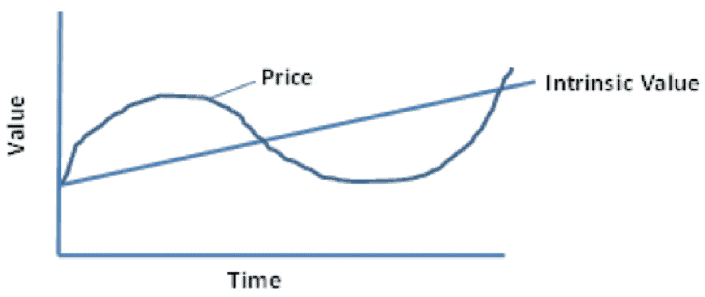
This picture defines a full economic cycle or asset class cycle such as a property cycle. We buy a property and hold it through the cycle believing that its value will rise 10% per annum. The price climbs with an exuberant market (freely available cheap mortgage debt), the property bubble bursts and property prices crash, interest rates rise and mortgage finance dries up. Banks start to lend again, property prices recover and, as long term buy and hold investors, we see our 10% expected return realised. The short term investor will have normally sold after the crash and missed the recovery.
Who Can Be A Long-Term Investor?
Most individual investors need the money to live on and so must be short term investors. They cannot take the chance of not having the money fully liquid and available to them “in case they need it.” That defines the situation and mind-set of the losing investors who generally donate their under performance to the longer term investor who calls it out performance. Many asset managers are also short term as their individual and institutional investors can ask for their money back any day or within a month or quarter for the longer term fund structures. So they have to invest for the short term. Hence most liquid active asset managers under perform their own indices as the longer term investors take performance from them.
Endowments, Foundations and Pension funds are most able to be true long term investors as there can rarely be a surprise event that requires them to liquidate investments. Foundations with 5% spending rules can lock up 95% beyond one year or 65% beyond 7 years (7 x 5% per year) theoretically. For school endowments, it depends on how dependent the school is on the endowment for meeting operating and capital expenditures. But most have 4% annual spending which points to situations not dissimilar to foundations. Pensions usually earmark liquid assets for near-term benefit payments which are well known and they lock up the rest for long term investment. So not surprisingly, endowments, foundations and pension funds, as a group, outperform high net worth investors and liquid asset managers as investors. But to take advantage of their unique status as long term investors, they must invest like long term investors, locking up capital and earning the so-called illiquidity premium available from investing with managers who invest for the long-term or into asset classes like private equity and property which lock capital up for 7-12 years but return some of the most attractive returns across all asset classes.
7. Market Returns (beta) vs. Manager Excess Returns (value added or alpha)
Investing can be broken into two different arenas:
Beta Arena: only take market risk through passive investments and get paid for it over the long term.
Alpha Arena: investing actively and taking a long term perspective to maximise chances of winning, taking a larger share of the investment pie. No investor has to play in the Alpha Arena and compete for a share of the pie. Any investor can sit that out and just accept that they may not be good at that. Logically, any purely short term investor should not play in the Alpha Arena, as they will most certainly be the loser. They should only play in the Beta Arena.
Playing only in the Beta Arena is easy in this age of cheap passive index tracking investment vehicles. For example, if you invest in a high risk index fund of small cap equities, you will earn what everyone else investing in that market is earning. You don’t win or lose. You just play for the market’s average long term return. And over the long term, that should be a positive number that is in proportion to the amount of risk you took. But you will not have handed over any of your money to the successful active investors who are winning a larger share of the pie or to high fee charging short term asset managers. In the Beta Arena, you take no risk that you will under perform (or over-perform). By playing in Alpha Arena, you do take that risk. And you have the choice not to play there. That choice should be made based on your long term investment horizon and your access to great long term investing asset managers.
With this clear delineation of the Beta Arena (the market risk only) and Alpha Arena (the risk of under performing the market) investors can track performance from what the market alone is doing for their portfolio returns (Beta returns) and what investment skill (whether yours or a that of a fee-charging asset manager you have entrusted) is doing to returns (Alpha returns). If playing in the Alpha Arena, any performance over or under what the Beta returns alone would have been, is the Alpha return (positive or negative).
This is the way we always report client investment performance. Break the total portfolio return into beta return and alpha return. If alpha return is consistently zero or negative, it is time to only play in the Beta Arena.
8. The Futility of Market Timing
Sadly, all too much of intelligent human kind are devoting their productive ingenuity to investing. Probably 5% or more of most developed economies are devoted to making markets more efficient by seeking to have insights others do not have. The result is that having an insight is very rare. Keeping in mind that 90% or more of this pool of human resource is focused on short term investing, the single investment decision that most of investment humanity are trying to get right is “when to get in and when to get out of the financial markets.” As a result of such intense focus on this one decision, so very few are able to get this right. We see the “risk on or risk off” decision as the single most difficult decision to get right. So we don’t try and do not think our clients should either.
We believe that most investors in fact get this wrong as they try to stem losses after most have run and then generally miss the recovery. This is what we call the risk exposure performance “leakage.” Our aim is to not allow our portfolios to leak any performance from bad market timing decisions. To ensure that we achieve this goal, we must know what the risk budget is for any given client, get the portfolio to that risk level and hold it there. Holding it there is not as easy as it sounds as active asset managers very often inadvertently move in unison adding or subtracting risk and leaking performance in our clients’ portfolios. We therefore monitor the overall look-through risk level and keep it level and avoid any performance leakage.
Keeping it level often has performance enhancing benefits. When risky assets decline in value, safe assets (like government bonds) usually increase in value. The result is that the portfolio’s overall risk level declines. We will at that time “rebalance” client portfolios back to their risk target by selling safe assets and buying risky assets right after the risky asset market decline. This has the same effect as we discussed earlier where panicky short term sellers are selling risky assets (e.g. equities) after they just got cheaper. We are the buyers from the panicky sellers, buying cheap in the name of just rebalancing to our target risk budget. Over the long term, this rebalancing activity tends to add up to 1% per annum in improved performance.