Article
The After-Tax Investment Lens: The Key to Tax Efficient Investing (California Taxpayer Version)
By Stan Miranda, David Shushan
28 Sep 2019
Note: This whitepaper has been explicitly written for California tax payers – the highest tax rate payers in the U.S. However, the lessons are highly applicable to U.S. taxpayers regardless of in which state they reside.
When investing, taxes matter more than you think and more than you would like. For wealthy Californians, it just got worse as state tax, the highest in the country at 13.3%, lost the bulk of its deductibility against federal taxes. Adding together federal, state, and Obamacare (Net Investment Income; “NII”) tax, translates into a maximum rate for ordinary income of 54% and a maximum rate for long-term capital gains of 37%. At the same time, projected asset class returns are declining. Accordingly, we believe optimization of after-tax investment returns has become an even more critical element of portfolio management for taxable investors.
This white paper summarizes our learning from many years of research and experience in optimizing after-tax return for US taxpaying clients. We start with an explanation of how taxes impact typical portfolios and then we lay out our five-step process for optimizing after-tax investment returns. Partners Capital was founded 18 years ago to bring what we believe to be the most advanced institutional investment approach to our clients. The foundation of this approach (often referred to as “the endowment model”) is multi-asset class diversification. Many “alternative” asset classes are relatively tax inefficient. “Alternatives” are often riddled with tax complexities that must be carefully understood. While many US investors have embraced the endowment model, we find they have not always properly accounted for these tax inefficiencies. Many clients we encounter in California have taken the attitude that after-tax returns will “all come out in the wash” by targeting the highest pre-tax returns, which is simply untrue. For example, at the extreme you could find yourself paying over 70% taxes on certain hedge funds classified as “investor status” as you pay taxes on returns gross of management fees (i.e. management fees are not deductible). Careful optimization of after-tax performance in an endowment-style portfolio increases annual post-tax returns nearly 30% (+1.2% annual incremental post-tax returns) compared with what could be achieved by ignoring taxes and optimizing pre-tax performance. Specifically, we project a 7.5% endowment style return, typical for today’s sophisticated investors focused on pre-tax results, will be taxed at 44%, delivering an after-tax return of 4.2%. When we set out to maximize post-tax returns, we believe private clients can achieve a 5.4% after-tax result(1).
This incremental return approaches the significance of the full +1.8% of total annual out-performance (alpha) generated by leading institutional investors such as the Yale endowment. Without a clear tax optimization plan, all the effort that goes into generating pre-tax out-performance through sophisticated investing can be erased by ignoring taxes. Our goal is to maximize expected after-tax results from a multi-asset class portfolio with a relatively high level of certainty. To do this, we have developed the following five.
Golden Rules of Tax Efficient Investing:
1. Focus on and measure after-tax performance
2. Increase portfolio risk to reflect the dampening effects of taxation
3. Allocate across asset classes based on after-tax returns, volatility and correlations
4. Select asset managers based on a range of after-tax expected returns
5. Utilize tax efficient structures
In Figure 1, we more fully define the five Golden Rules and their contribution to the potential improvement in post-tax returns.
Figure 1: Summary of Five Golden Rules of Tax Efficient Investing
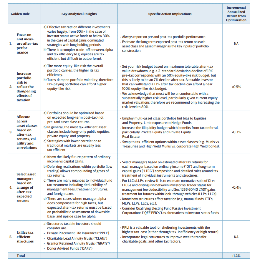
Figure 2: US Taxable Client Checklist
Individual tax paying clients should review their portfolios across the following key areas to improve tax efficiency.

How Taxes Presently Impact California Tax Payer Portfolios
Over the past ten years tax rates have climbed and are taking an increasingly large share of investment portfolio gains. At the same time, slow economic growth, quantitative easing and low interest rates worldwide have decreased forward looking returns across asset classes. The result is an environment where post-tax take-home investment gains have eroded. When considering inflation, the impact on real after-tax returns is even more dramatic.
At the federal level, tax rates for short-term capital gains are up from 35% to 40.8% and long-term gain rates have risen from 15% to 23.8%, including the 3.8% Net Investment Income (NII) “Obamacare” Tax. While the 2017 Tax Cuts and Jobs Act decreased the top federal tax rate from 39.6% to 37%, we expect most wealthy California income earners will see minimal
benefit or even an increase in their effective rate due to reductions in allowable deductions and the $10,000 cap on state and local tax (SALT) deductions (2). This is particularly hard-hitting as California has the highest state tax in the country, at 13.3%. For example, for California tax payers in the top state and federal brackets for annual income saw their tax rate on income increase by 12.4% from 2008 to 2018 given the increase in state taxes from 2009-2012 and the cap on SALT deductions from federal taxes in 2017.
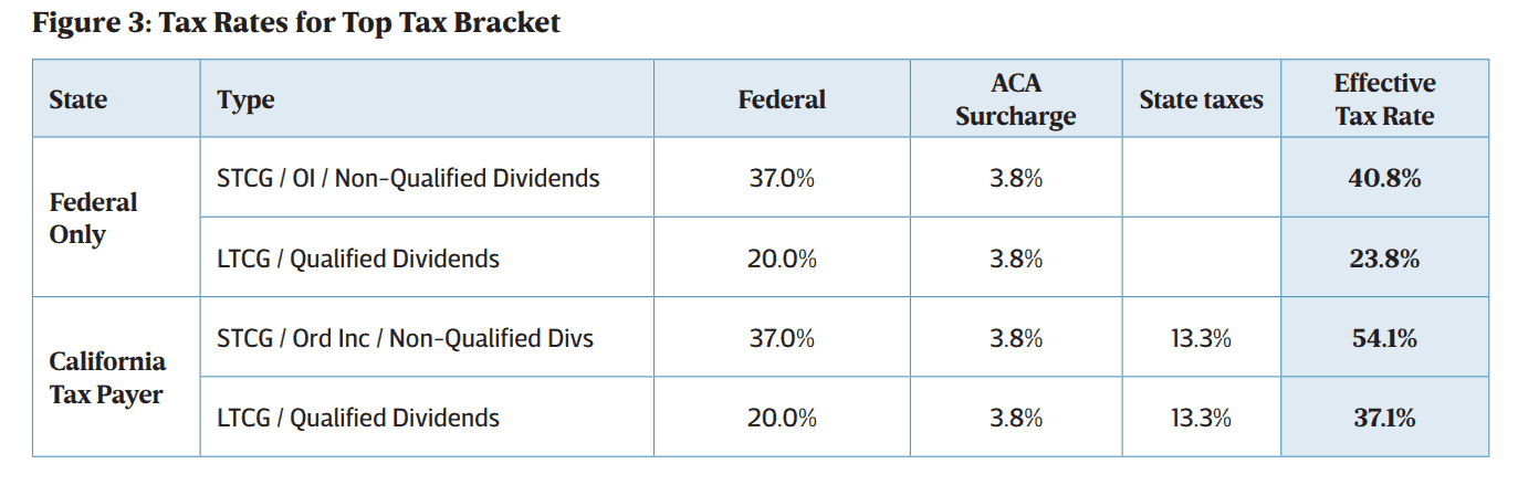
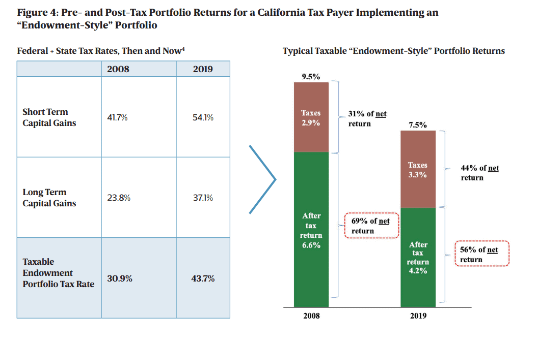
When you put all these taxes together for Californians, as seen in Figure 3, short-term capital gains, ordinary income, and non-qualified dividends are taxed at a maximum rate of 54.1%. Long-term capital gains and qualified dividends are taxed at 37.1%; hence a 17% spread between short-term and long-term capital gains treatment. This means a portfolio implementing the asset allocation of a typical endowment-style portfolio will give away almost 44% of gains in taxes, inclusive of the state levy, up from 31% taxes 10 years ago, as seen in Figure 4. The tax increase has occurred coincident with an environment where expected returns have fallen across asset classes, exacerbating the impact. We estimate that today’s typical endowment-style multi-asset class portfolio has an expected pre-tax return of 7.5% (3) . This is down from 9.5% annualized pre-tax return ten years ago, as shown in Figure 4. The decrease in returns, in conjunction with higher tax rates means that after-tax annualized results have declined over 35%, from 6.6% in 2008 to 4.2% today, as shown in Figure 3. Subtracting inflation of 2%, real after-tax results have been cut in half, from 4.6% to 2.2%.
Below, we lay out our five golden rules for optimizing after-tax returns short of leaving the state of California and moving to no or low taxing states such as Nevada, Florida and Texas.
Golden Rule #1 – Focus on and Measure After-Tax Performance
Without a deep understanding of a portfolio’s tax consequences, it is unlikely that investors will do what they need to do to preserve and grow the base of assets through maximizing real after-tax returns. It is not easy to measure after-tax returns. For example, there are issues with the reporting and calculation time lag, the interaction of investment taxes with taxes on earned income or non-financial assets outside the portfolio, and a range of other factors. Despite these challenges, we believe it is possible to arrive at useful forward-looking estimates of tax impact on various investments and on your overall portfolio.
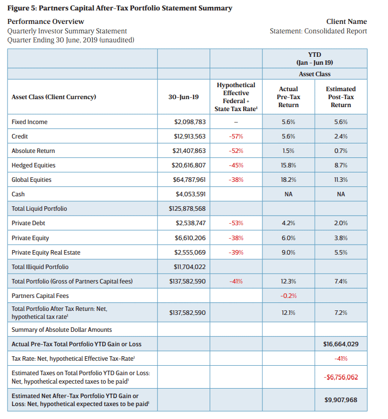
Figure 5 shows a typical summary page for one of our taxable Californian clients, reflecting both the pre-tax and hypothetical post-tax return. We build up and report expected portfolio tax estimates through an analysis of the expected tax rate on the underlying investments in the portfolio. These estimates are used to adjust the pre-tax return on a statement to create a hypothetical post-tax return(5). In the sections that follow, we explain more thoroughly how we arrive at these estimates. At Partners Capital, the summary performance report, as shown in Figure 5 takes asset class tax rates from the sum of our estimates of each underlying asset manager’s likely tax treatment. Any approved asset manager is analyzed for tax treatment (based on review of past K-1s and similar information) and we log the expected tax treatment of income and gains in our systems. We can compare the aggregate tax rate and expected after-tax returns to a passive portfolio to ensure there is enough projected alpha to offset the higher tax rate of an endowment-style approach. For example, if a passive portfolio is expected to deliver a 5% return with a 25% tax rate (3.8% after-tax) and an active portfolio is expected to deliver a 7.5% return with a 44% tax rate (4.2% after-tax), then we know that any tax inefficacies are offset by superior active manager performance.
Using these estimates, we can isolate asset classes where investment managers are more or less efficient than their asset classes (represented passively) and put a spotlight on which allocation decisions or investments are contributing the most and least to after-tax returns for the overall portfolio.
Golden Rule #2 – Increase Portfolio Risk to Reflect the Dampening Effects of Taxation
Thinking of your risk budget in terms of maximum after-tax drawdown or volatility may point to increasing your overall portfolio risk level. Our tax paying clients with a true long-term investment
horizon are taking on approximately 20% higher risk once they examine risk in after-tax terms. This type of risk increase (e.g. going from 63% equivalent equity risk to 80%) is expected to add
+0.5% to after-tax results, moving annual returns from 4.2% to 4.7%6. The risk budget in a portfolio is one of the most important decisions that investors make. Traditionally, taxable investors focus on pre-tax return volatility and drawdown levels to set risk budgets. Taxation has a volatility-reducing effect on returns in both up and down markets. Most investment portfolio value declines manifest themselves in the form of realized or unrealized capital losses, rather than ordinary income losses. In the event of a capital loss in a given year, the portfolio will carry a loss forward into the following year, which is used as a credit against future gains. This credit dampens the actual after-tax downside experienced by creating an asset to be used in the future. We believe that taxable investors should focus on post-tax volatility and drawdowns to establish their risk budgets.
Investors generally set the maximum amount of risk they want to take in their portfolios (i.e. their “risk budget”) in terms of the maximum decline in portfolio value or drawdown at any point in time or over any given period – usually one year. One way to estimate this maximum drawdown is to think about how investment returns have varied in the past as measured by the standard deviation or volatility of their returns. Historically, annual public equity market return volatility has averaged around 16% with an average return of 9%, therefore, we would expect annual returns for two of three years to fall between -7% and 25%, if the returns were normally distributed. We characterize the maximum drawdown tolerable for an investor as a two-standard deviation move below the expected return, which we would expect to happen once in 40 years (and two standard deviation above the expected return once in 40 years). So, thinking just about public equities, with most experts forecasting future public equity returns of 6% per annum, the two standard deviation downside outcome would be a -26% decline in value (6% expected return minus 2 x 16%). Most investors are not comfortable with the prospect of a -26% decline and set risk budgets below 100% equity-like risk, whether they pay taxes or not. Assuming an average tax rate of 44%, the comparable two-standard deviation aftertax decline of public equities is -14.6% (3.4% expected after-tax return minus 2 x 9%). Clearly a maximum drawdown of -14.6% is more acceptable than a maximum drawdown of -26%, which underscores the importance of setting portfolio risk budgets in terms of maximum after-tax drawdowns. We use Figure 6 to make the case for a tax paying investor to take greater risk than a typical nontaxable endowment portfolio. We use a measure of equity like risk to discuss risk budgeting – specifically equivalent net equity beta (ENEB). Most of us can relate to what the risk of a pure 100% public equity portfolio would be, especially if we believe the historical average annual volatility of 16% to be a useful guide. As a starting frame of reference, the average non-taxable endowment investor in the US takes on about 63% of the risk of a pure equity portfolio or a 63% ENEB. As shown in Figure 6, this translates into a theoretical maximum drawdown of -12.5% in a given year. For taxable investors comfortable with a maximum theoretical post-tax drawdown of -12.5%, the portfolio’s equity-like risk can be hypothetically increased to 100% assuming an effective tax-rate of 44%. If investors truly set their personal risk budgets based on after-tax drawdown potential, they would be raising risk budgets as tax rates rise. We rarely see this.
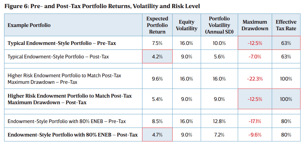
In our tax-optimized asset allocation for US tax payers, we recommend 80% equity-like risk, which is ~20% higher than the typical tax-exempt endowment-style asset allocation which has around 63% equity-like risk. While risk budgets for large taxable family offices and ultra-high-net worth individuals vary considerably, the mean risk level we observe most often is very close to this 63% level (usually sitting between 50-70% equity-like risk). While simply adjusting a typical institutional portfolio risk level for the effects of taxes would point to a risk budget of something close to 100%, we find that our typical tax-paying clients usually stop short of moving their portfolios to the full risk level required to equate pre- and post-tax drawdowns. We chose 80% to acknowledge the fact that taxes reduce the volatility of investment returns suggesting that higher risk is appropriate for taxable investors. Offsetting this, however, we need to reflect the fact that most taxable individual investors do not have the same long-time investing horizon and same risk appetite as typical nontaxable institutional investors. Hence, we use an equitylike risk budget of 80% to illustrate the portfolio return impact of moving up the risk spectrum from where we typically see the wealthiest tax-paying individuals. Using our models for optimal asset allocation, which optimize for the best risk-adjusted after-tax returns, we estimate that an increase in risk budget from 63% to 80% adds 0.5% to the expected multi-asset class portfolio after-tax return, increasing it from 4.2% to 4.7% as shown above.
Golden Rule #3 – Allocate Across Asset Classes Based on After Tax Returns, Volatility and Correlations
Optimizing a multi-asset class portfolio for a higher level of equity-like risk improves after-tax results by an incremental +0.3% bringing after-tax returns from 4.7% to 5.0% (7).
The most basic asset allocation optimization model is the Markowitz mean variance optimization model which has three key inputs for each asset class: expected return, standard deviation of returns and correlations of returns with other asset classes. At Partners Capital, we run these models as one input to a more judgemental asset allocation process. But, critically, we build tax-paying client portfolios using a totally different set of inputs for these three factors by adjusting them for after-tax returns. After-tax returns (7) are of course lower, but they decline by varying
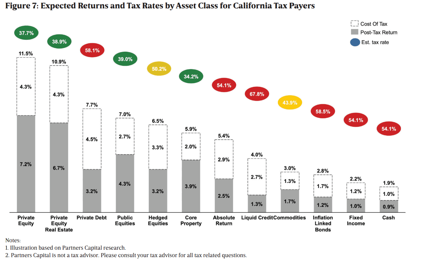
amounts depending on tax efficiency of any given asset class. Figure 7 shows our projected pre- and post-tax returns by asset class incorporating both federal and California state taxes. The tax rates are derived from the typical mix of ordinary income vs long term capital gains for each asset class applied to expected future average returns including a modest amount of expected out-performance or alpha from active management. The tax rates applied to each asset class are what we see as the typical manager’s tax treatment, not the most tax efficient manager or strategy within each asset class. Those savings are discussed below under Golden Rule #4 which focuses on asset manager selection as a source of further improvement of after-tax returns. To improve the overall tax efficiency of our taxable portfolios, we bias them toward tax advantaged asset classes such as public equities, private equity and real estate. In addition, we consider municipal bonds in place of Treasuries and structured inflation-linked municipal bonds (municipal bonds plus a return swap linked to the Consumer Price Index) in place of traditional inflation-linked bonds. Conversely, we avoid tax-inefficient asset classes with low manager out-performance (alpha) potential such as liquid credit and are selective on absolute return and hedged equities.
The least tax efficient asset classes are yield-based including liquid credit, inflation-linked bonds, traditional fixed income (such as Treasuries) and private debt because the income stream is subject to the higher ordinary income tax rates. Absolute Return strategies are usually highly tax-inefficient as well given the high frequency of trading inherent to many uncorrelated strategies. Hedged Equities are marginally better (50.2% effective tax rate) but suffer from high turnover leading to mostly short-term capital gains which are taxed at ordinary income tax rates. Both liquid public equities and private equity which are held (and not realized) for long periods of time have low effective tax rates due to the benefits of deferral, as unrealized gains accumulate tax free and returns compound on those unrealized gains. Property (particularly core property) is among the most tax efficient asset class with a 34.2% expected tax rate. This is primarily because depreciation, capex and interest expenses shield ordinary income generated by tenants, allowing investors to defer taxes to the point of sale, at which point they are recaptured at a reduced rate (38%) up to the property’s cost basis. Gains beyond the cost basis are fully deferred and taxed at long-term capital gain tax rates. Taxes on some property gains can be completely avoided in Section 1031 exchanges where you sell an investment property and reinvest the proceeds from the sale within certain time limits in a property or properties of like kind and equal or greater value.
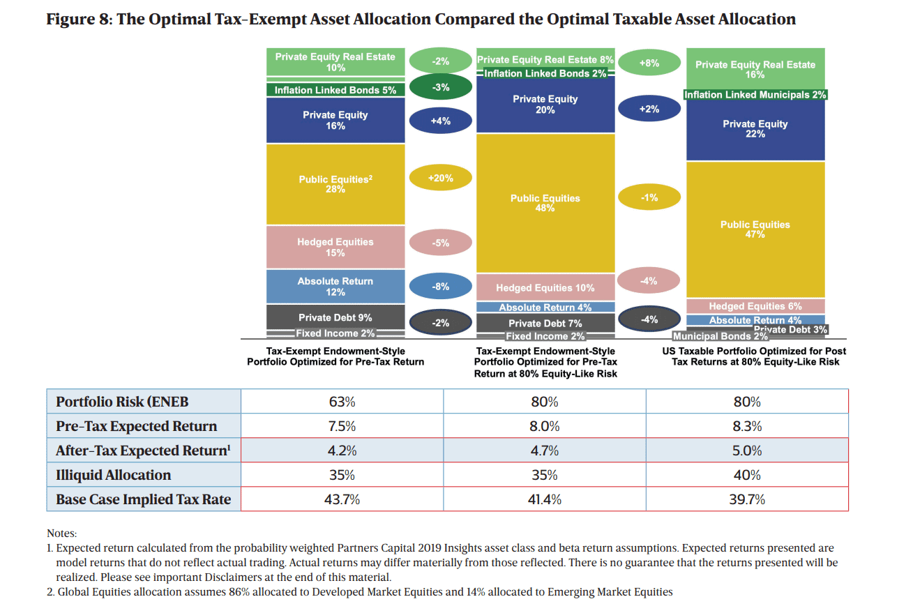
Below in Figure 8 we compare our recommended non-taxpaying institutional client portfolio with an equity-like risk budget of 63% to the optimal asset allocation for a non-tax paying client with an equity-like risk budget of 80%. You can see that this adds 0.50% to the expected return as discussed under rule #2 above. The third bar (far right) then incorporates the after-tax returns of each asset class to shift from what is an optimal mix for a non-taxpayer to what is optimal for a California tax paying investor. It emphasizes tax efficient asset classes such as private equity, global equities and real estate, which comprise three-quarters of the asset allocation, while reducing investments in private debt, absolute return, and inflation linked bonds.
Relative to the higher risk asset allocation optimized for non-taxpaying investors, the higher risk tax optimized portfolio for California tax payers results in a 39.7% effective tax rate compared to a 41.4% effective tax rate, adding +0.3% to after-tax returns (from 4.7% to 5.0%).
Golden Rule #4 – Select Asset Managers Based on a Range of Expected After-Tax Returns
The legal structures and strategies of individual asset managers have a material impact on after-tax returns. By appropriately analyzing the tax consequences of alternative asset managers and selecting asset managers based on their expected after-tax returns, it is possible to further improve after tax returns by +0.4% to 5.4%(8).
We find that few investors select managers based on their expected after-tax returns relative to their peer group. Tax advisors know how taxes affect different asset managers, but they don’t know how to estimate expected pre-tax returns. Investment advisors should be good at estimating an asset manager’s expected pretax return in the future, but most do not understand the likely after-tax outcome. At Partners Capital, we work with tax advisers to apply their knowledge on taxes to our knowledge on expected pre-tax returns to arrive at the best view for selecting asset managers. With this knowledge, we put in the effort to understand each asset manager’s tax profile as defined below.
Vehicle Type and Legal Structure-Based Tax Savings
Investments come in the form of directly held public securities, futures and options and directly owned private companies, private debt and private property. Most large investors invest much of their capital via third party managers or instruments including mutual funds (Reg 40 Act funds), exchange traded funds (ETFs), real estate investment trusts (REITs), Master Limited Partnerships (MLPs) and look-through vehicles including limited liability companies and partnerships (LLCs and LLPs), to name a few. Investments can be on-shore or off-shore.
Each of these will have a different mix of long-term capital gains, short-term capital gains, qualified dividends and other ordinary income and may be taxed on a lookthrough or non-look through basis. So it is complicated, but it is worth the effort to know how each are taxed.
Four of the most important concepts in understanding investment vehicle tax efficiency are:
1. The normative mix of long-term capital gains,short-term capital gains, qualified dividends and other ordinary income.
2. Realized versus unrealized gains – the benefit of tax deferral from long hold periods
3. Investor vs. Trader status LLCs or LLPs – determines deductibility of fund management fees and other expenses
4. Gains on futures / Section 1256 gains – where all gains are considered fully realized (annually) with 60% long-term and 40% short-term capital gains treatment
1. Normative mix of LTCGs, STCGs, qualified dividends, other ordinary income and deductible expenses
Most investors know that their tax advisors need to closely examine past form 1099s for mutual funds and K-1s for look-through vehicles to estimate the future taxes on such investments. K-1s are more complicated with gains and income spread throughout the document and varying from one year to the next. It is important to examine at least three years of K-1s to arrive at reasonable assessments of historical tax charges as a basis for forecasting the future.
2. Realized versus unrealized gains – the benefit of tax deferral
Portfolios that derive their return from capital gains, which are only paid on realization, benefit from the impact of deferral. Deferral is a highly effective means of tax rate reduction. While a powerful tool, tax deferral is not tax elimination except in the case of holding beyond one year where long-term gains taxation is -17% lower than short-term gains taxation.
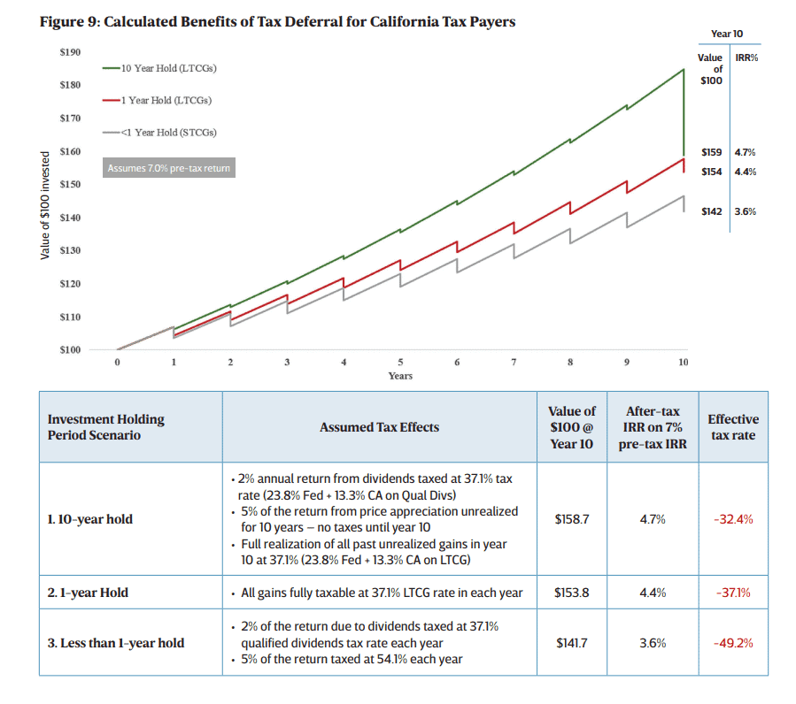
When you defer gains by not selling securities in any given year, the IRS, in effect, lets you keep the taxes which will eventually be owed and accrue income and gains on gross-of-tax assets at work. In this way, deferral reduces the effective tax rate on long-term gains by allowing multi-year compounding of untaxed returns. As shown in Figure 9 below, the impact of deferral is even more pronounced when looking through the lens of paying short-term capital gains on most of the pre-tax returns, where the benefit to only paying long-term capital gains taxes on 2% of the pretax annual return translates to a 17% lower effective tax rate over 10 years.
It is important to note that LLPs and LLCs will “pass through” the realized gains and losses from underlying trading activity to their investors, regardless of whether the investor has taken any action in the fund (e.g. trimmed or added, received a dividend, etc.). For example, if a stock is sold at a gain within such a fund, the gain from the sale is reportable for the investor as a taxable gain in that year via K-1 reporting. This means that taxable gains and loses can differ from economic gains and losses (money in your pocket). Ultimately, realized and unrealized gains converge, but only over the life of the investment (5 – 15 years). Many offshore funds are deemed to be Passive ForeignInvestment Corporations (PFICs) which have punitive tax consequences unless a “PFIC letter” is obtained from the offshore fund sponsor. A Passive Foreign Investment Corporation letter, or PFIC letter, if offered by the fund, shows the capital gains and/or income attributable to their position in the calendar year. Note that PFICs will not show realized losses, therefore losses on one’s investment are carried forward within the fund and cannot be used to offset gains elsewhere in a taxable portfolio. If an investor redeems the position at a loss, the losses are realized and are offsettable against gains in the portfolio at that time. For the IRS to characterize the gains on a PFIC as capital gains and income, the investor in the PFIC must elect that the PFIC is a qualifying electing fund (“QEF”) otherwise all income from the PFIC is characterized as ordinary income and interest costs can be charged. Given the many complexities and onerous burdens for misfiling elections, it is only in rare instances that a taxable investor would invest in a PFIC.
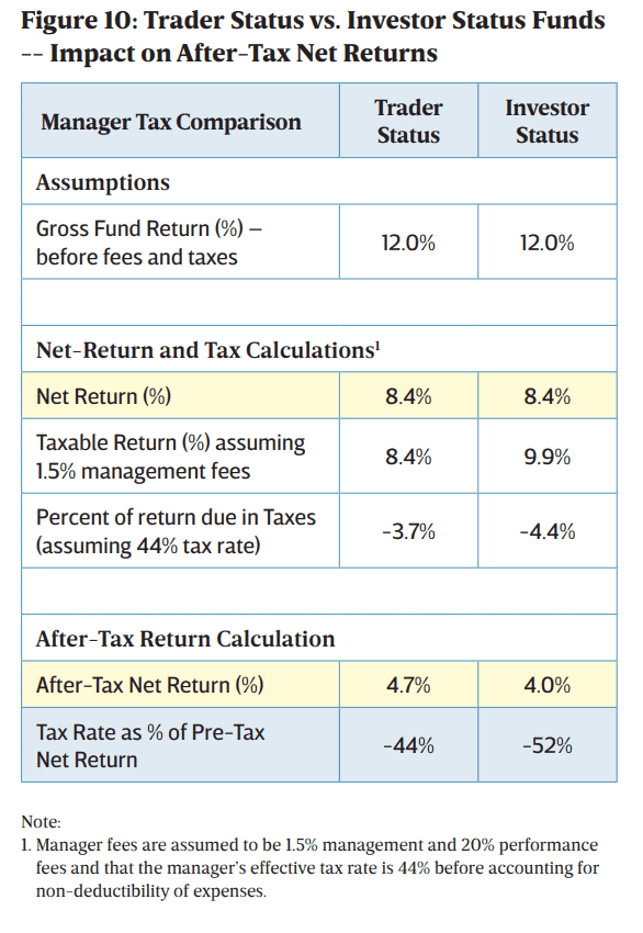
3. Investor vs. Trader status – deductibility of fund management fees and other expenses Fees and expenses generally reduce the taxable investment return except in some cases with look through vehicles such as LLCs and LLPs. Mutual funds, ETFs, REITs and other similar investment vehicles allow for all expenses to be offset against their underlying income and capital gains for tax calculations. The tax status of LLCs and LLPs is an annual determination made by the auditor of the fund, based on the degree to which the fund trades the underlying investments. If a fund is classified as “investor status” (versus “trader status”) then management fees and certain other expenses are not deductible against gross investment income for income tax purposes. The result is that taxes are charged on returns net of performance fees but gross of management fees. This is particularly costly for investor status funds with high management fees and low returns. Figure 10 highlights the potential for an investor status fund to have an 8% higher effective tax rate versus a trader status fund with the same underlying return and tax-rate assumptions.
Typically, we find strategies which hold onto the underlying assets for long periods (“long-hold funds” e.g. private equity, private debt, long equities, and certain hedge fund strategies) are classified as investor status. Higher frequency trading funds (e.g. absolute return, quantitative, and some hedge fund strategies) will generally be classified as trader status, because they are considered to be in the “trade or business” of trading stocks. In both investor and trader status funds, performance fees (or carried interest) reduce the taxable gain and are therefore not taxed and are effectively “deductible.” Only management fees and other expenses of the fund are not deductible in the case of investor status funds. In the case of a lower-returning investment or one that has higher management fees, the effective tax rate can easily go above 50% and sometimes reach over 100%. Credit managers structured through LPs / LLCs focusing on taxable bonds often fall into this category and effective tax rates often reach 70% or higher.
As noted above, PFICs only report capital gains and ordinary income on a net asset value basis. Therefore, management fees are netted against ordinary income and are essentially tax deductible. This can improve the effective tax rate for funds with high management fees and low performance results. US taxpayers allocating to investor status funds may consider allocating to the offshore equivalent if the fund allows onshore investors, issues appropriate PFIC letter and can qualify for a QEF declaration.
4. Gains on futures / Section 1256 gains – where all gains are considered fully realized (annually) with 60% long term and 40% short term capital gains treatment
The attractiveness of using futures depends on the asset class and strategy being undertaken. In the instance of US Treasuries, it can be attractive to use futures in lieu of direct bonds as investors would hypothetically pay 60% long term and 40% short term rates on gains from the futures compared to gains being fully taxed at income rates for cash Treasuries, assuming that yield is the only component of forward-looking returns. Alternatively, using the example of global equities, it is less attractive to hold equities futures as the 60% / 40% treatment is significantly worse than the buy-and-hold cash equities strategy which have something closer to 100% taxes at LTCG rates (including the qualified dividends).
Optimizing After-Tax Returns Within Each Asset Class
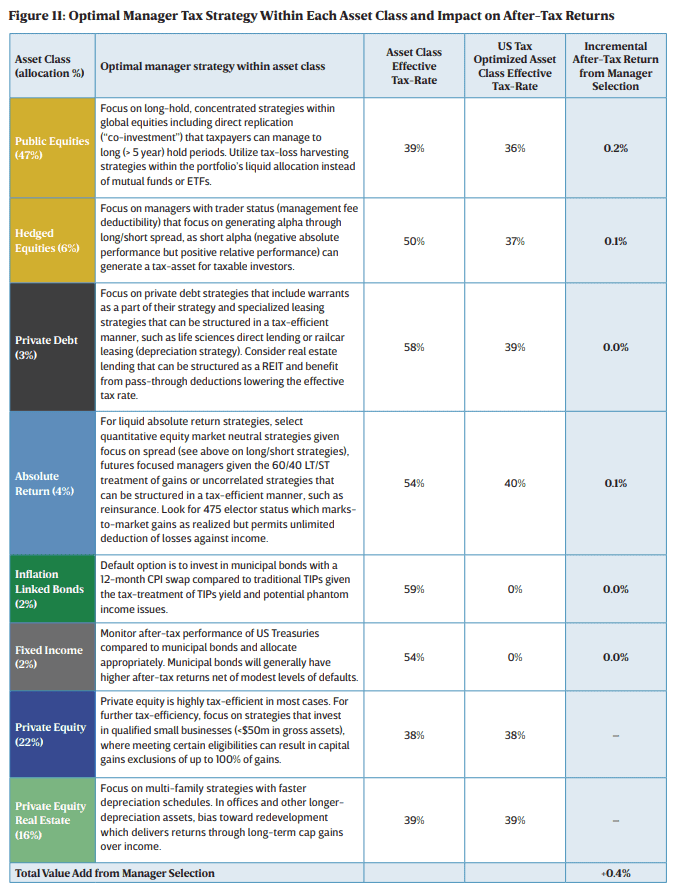
In Figure 11, we lay out what we believe to be some of the most effective tax strategies for optimizing the post-tax returns of each asset class. The greatest opportunity for tax savings in manager
selection is generally found in public equities from the combination of long hold strategies and tax loss harvesting. We discussed long-hold strategies above. Tax loss harvesting is the practice of selling a security that has experienced a loss. By realizing, or “harvesting” a loss, investors can offset taxes on both gains and income. The sold security is replaced by a similar one, maintaining an optimal asset allocation and expected returns. Tax loss harvesting benefits deteriorate over time as gains become embedded in the portfolio and harvestable losses become scarcer. This is due to the strategy systematically selling stocks with losses and retaining stocks with gains, therefore, if the market continues to rise then generally there will be fewer positions with losses to sell and more with imbedded gains which will not be sold. In addition, loss harvesting over time increasingly runs the risk of tracking error against its benchmark as the positions purchased from the sale of stocks with losses cannot be identical to the position sold or the losses generated would be disallowed under wash-sale rules.
Selecting Managers Where Alpha More Than Compensates for Tax Inefficiency
While we often look to select managers that improve upon asset class selection, in many cases the returns of an individual manager can more than compensate for any tax inefficiency in its strategy and/or asset class. Selecting a manager with lower tax-efficiency but higher post-tax alpha requires conviction in the forward-looking pre-tax alpha expectations. Included in Figure 11 are our estimates of where we believe investors are likely to be making the wrong tradeoff by passing on high performing managers. We acknowledge that many investors may not be making this mistake, but we feel it is useful to illustrate a few examples where manager outperformance may justify paying the higher taxes.
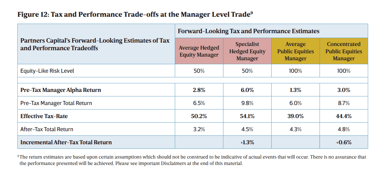
Quite simply, we want to stress here how critical it is to think about tax rate and total returns in combination. In some cases, the returns on an individual manager can more than compensate for the tax inefficiency. An example of this includes specialized managers within the Hedged Equity asset class, where we believe that expert knowledge within a geography, sector or sub-sector will lead to higher than the asset class average pre-tax alpha generation. Another exceptional instance would be a concentrated Public Equities manager that structures its largest positions in a manner to maximize returns while mitigating potential downside through derivatives. The structuring may result in gains being characterized in less tax-efficient manner, but the additional tax cost is more than offset by the higher alpha generation from the structuring. Figure 12 illustrates this effect. By optimizing strategy and fund selection using the factors above, we expect that we can reduce the portfolio’s effective tax-rate by -2.4% and add an additional +0.4%(10) in after-tax results to portfolios versus a portfolio with an average (as defined by tax rate in the asset class) fund line-up.
Golden Rule #5 – Utilize Tax Efficient Structures
Any good tax strategy must examine the various legal structures that may be pertinent to the private investor’s personal situation and provide for far more substantial income tax savings than the recommendations described above. The list of tax structuring options is long and requires the engagement of specialized tax counsel. Below we provide you with a shorter list of examples of tax efficient structures that Partners Capital clients have deployed most frequently with our clients.
These include Charitable Lead Annuity Trusts (“CLATs”), Grantor Retained Annuity Trusts (“GRATs”), Donor Advised Funds (“DAFs”), and Private Placement Life Insurance (“PPLI”). Figure 13 provides a brief description of each of these four tax efficient structures with a description of the intended benefits.

In recent years, Private Placement Life Insurance (“PPLI”) has seen significant improvements in the overall cost of insurance and better definition around the rules that govern it, making it a very powerful tool for certain portfolios looking to pass assets to their heirs in a tax efficient manner. Partners Capital has been involved in helping clients with PPLI underlying investments for many years and today operates a range of insurance dedicated funds mostly focused on housing the most tax inefficient but higher returning investment strategies.
Charitable Lead Annuity Trusts (“CLATs”) and Grantor Retained Annuity Trusts (“GRATs”) benefit from the current low interest rate environment, as the annual distribution requirement is tied to an interest rate determined by the IRS, potentially leaving a higher percentage of the trust’s assets that can be transferred to beneficiaries after the period of charitable payments has expired.
For charitable giving, the use of Donor Advised Funds (“DAFs”) can be advantageous over setting up a private foundation. The trade-offs individuals should consider regarding DAFs are higher itemized deduction rates (60% of AGI vs 30% of AGI), lower program taxes and expenses, and a lower administrative burden compared to a private foundation. The primary trade-off with DAF’s is a reduced universe of investment options as you are limited to what the DAF manager offers.
For DAFs, individuals can currently deduct cash contributions of up to 60% of their annual gross income (“AGI”) at the time they make their contribution to a DAF, which is higher than the limit of 30% for cash contributions to a private foundation. Non-cash contributions, such as stock contributions, are capped at a lower amount, specifically 30% for non-cash contributions to a DAF and 20% for non-cash contributions to a private foundation. Furthermore, an individual can make an excess charitable contribution, defined as a contribution greater than 60% of AGI for a DAF or 30% of AGI for a private foundation in a given year. The excess charitable contribution can then be deducted annually over the subsequent 5 years until it is all used, subject to the maximum annual deduction limit as a percentage of AGI. For example, if an individual with $10m of AGI contributes $36m to a DAF, they can deduct the maximum amount of $6m in the year that they contributed to the DAF and then $6m annually for the following 5 years (assuming AGI remains constant). If that same individual chose to set up a private foundation, they could only deduct the maximum amount of $3m in the year that they contributed and then $3m annually over the following five years (assuming AGI remains constant, as above).
As a DAF is provided by a third party, the individual avoids any additional tax filings associated with the program, but typically limits the DAF’s investment portfolio to available investments on a third party’s platform. Private foundations provide additional flexibility for the program’s investment options, but often can be more expensive and time consuming than a DAF, especially considering the IRS Form 990PF filing requirements and annual 2.0% net investment income tax that is charged on private foundation’s investment income, but not on the income of a DAF.
Conclusion
We believe that an endowment-style of multi-asset class portfolio management continues to be the optimal investment strategy for private investors with substantial accumulated wealth and a long investment time horizon. Nevertheless, it must be modified relative to non-tax paying endowment portfolios to optimize after-tax returns. The simplest advice is that all key investment decisions – risk budget, asset allocation and manager selection – must be made based on after-tax expected risk and returns. Measuring and reporting on after-tax returns will help to reinforce this discipline.
We recommend taxable portfolios target higher equity-like risk levels than their tax-exempt counterparts (generally 80%-85%, and potentially higher) in consideration of the tax efficiency of
higher-risk assets and the volatility-dampening effects of taxes. We estimate that increasing the risk level by focusing on higher equity-like risk strategies could increase the after-tax return by +0.5% . In addition, we modify the asset allocation in favor of more tax efficient asset classes to improve post-tax returns by +0.3%11. By making more fully-informed and deliberate manager selection decisions, we improve post-tax results by an additional +0.4%(11). Taken together, we expect a well-optimized taxable portfolio can return 5.4%, which is a +1.2%11 improvement over a typical endowment-style multi-asset class portfolio. Incorporating additional overarching legal structures can help in wealth transfer or in achieving charitable goals. Too often, taxes are ignored because they are “invisible” to advisors, leading to sub-optimal decision-making and advice. In reviewing projected returns and actual results with taxable clients, the focus must be on what the investor takes home after taxes are paid.
Note: Partners Capital Investment Group, LLP is not a tax adviser. Clients should seek independent professional advice on all tax matters. Please see the important disclaimers at the back of this document for further detail.
1 The return estimates are based upon certain assumptions which should not be construed to be indicative of actual events that will occur. There is no assurance that the performance presented will be achieved. Please see important Disclaimers at the end of this material.
2 The removal of the SALT deduction may increase taxes for individuals previously subject to AMT (Alternative Minimum Tax), as they may now see a higher overall tax-bill than their previous tax-bill including AMT. For ultra-high net worth individuals, most were not paying AMT to begin with, therefore losing the SALT deduction has a direct impact as illustrated in the body of this document.
3 The return estimates are based upon certain assumptions which should not be construed to be indicative of actual events that will occur. There is no assurance that the performance presented will be achieved.
4 For the information shown regarding 2008 tax rates, the analysis assumes that long-term capital gains are the only source of taxable income. Additionally, the phase-out of itemized deductions has not been reflected in the rates shown for 2008.
5 Hypothetical post-tax returns do not represent actual trading. Actual post-tax returns may differ materially from those reflected. There is no guarantee that the hypothetical returns assumptions presented will be realized.
6 The return estimates are based upon certain assumptions which should not be construed to be indicative of actual events that will occur. There is no assurance that the performance presented will be achieved.
7 The return estimates are based upon certain assumptions which should not be construed to be indicative of actual events that will occur. There is no assurance that the performance presented will be achieved.
8 The return estimates are based upon certain assumptions which should not be construed to be indicative of actual events that will occur. There is no assurance that the performance presented will be achieved.
10 The return estimates are based upon certain assumptions which should not be construed to be indicative of actual events that will occur. There is no assurance that the performance presented will be achieved.
11 The return estimates are based upon certain assumptions which should not be construed to be indicative of actual events that will occur. There is no assurance that the performance presented will be achieved.